June 2012
When we discuss prediction models, prediction errors can be decomposed into two main subcomponents we care about: error due to "bias" and error due to "variance". There is a tradeoff between a model's ability to minimize bias and variance. Understanding these two types of error can help us diagnose model results and avoid the mistake of over- or under-fitting.
Bias and Variance
Understanding how different sources of error lead to bias and variance helps us improve the data fitting process resulting in more accurate models. We define bias and variance in three ways: conceptually, graphically and mathematically.
Conceptual Definition
- Error due to Bias: The error due to bias is taken as the difference between the expected (or average) prediction of our model and the correct value which we are trying to predict. Of course you only have one model so talking about expected or average prediction values might seem a little strange. However, imagine you could repeat the whole model building process more than once: each time you gather new data and run a new analysis creating a new model. Due to randomness in the underlying data sets, the resulting models will have a range of predictions. Bias measures how far off in general these models' predictions are from the correct value.
- Error due to Variance: The error due to variance is taken as the variability of a model prediction for a given data point. Again, imagine you can repeat the entire model building process multiple times. The variance is how much the predictions for a given point vary between different realizations of the model.
Graphical Definition
We can create a graphical visualization of bias and variance using a bulls-eye diagram. Imagine that the center of the target is a model that perfectly predicts the correct values. As we move away from the bulls-eye, our predictions get worse and worse. Imagine we can repeat our entire model building process to get a number of separate hits on the target. Each hit represents an individual realization of our model, given the chance variability in the training data we gather. Sometimes we will get a good distribution of training data so we predict very well and we are close to the bulls-eye, while sometimes our training data might be full of outliers or non-standard values resulting in poorer predictions. These different realizations result in a scatter of hits on the target.
We can plot four different cases representing combinations of both high and low bias and variance.
| Low Variance | High Variance | |
| Low Bias | ||
| High Bias |
Mathematical Definition
after Hastie, et al. 2009 1
If we denote the variable we are trying to predict as $Y$ and our covariates as $X$, we may assume that there is a relationship relating one to the other such as $ Y = f(X) + \epsilon $ where the error term $ \epsilon $ is normally distributed with a mean of zero like so $ \epsilon \sim \mathcal{N}(0,\sigma_\epsilon) $.
We may estimate a model $ \hat{f}(X) $ of $ f(X) $ using linear regressions or another modeling technique. In this case, the expected squared prediction error at a point $ x $ is:
$$ Err(x) = E\left[(Y-\hat{f}(x))^2\right] $$
This error may then be decomposed into bias and variance components:
$$Err(x) = \left(E[\hat{f}(x)]-f(x)\right)^2 + E\left[\left(\hat{f}(x)-E[\hat{f}(x)]\right)^2\right] +\sigma_e^2 $$
$$Err(x) = \mathrm{Bias}^2 + \mathrm{Variance} + \mathrm{Irreducible\ Error}$$
That third term, irreducible error, is the noise term in the true relationship that cannot fundamentally be reduced by any model. Given the true model and infinite data to calibrate it, we should be able to reduce both the bias and variance terms to 0. However, in a world with imperfect models and finite data, there is a tradeoff between minimizing the bias and minimizing the variance.
An Illustrative Example: Voting Intentions
Let's undertake a simple model building task. We wish to create a model for the percentage of people who will vote for a Republican president in the next election. As models go, this is conceptually trivial and is much simpler than what people commonly envision when they think of "modeling", but it helps us to cleanly illustrate the difference between bias and variance.
A straightforward, if flawed (as we will see below), way to build this model would be to randomly choose 50 numbers from the phone book, call each one and ask the responder who they planned to vote for in the next election. Imagine we got the following results:
| Voting Republican | Voting Democratic | Non-Respondent | Total |
|---|---|---|---|
| 13 | 16 | 21 | 50 |
From the data, we estimate that the probability of voting Republican is 13/(13+16), or 44.8%. We put out our press release that the Democrats are going to win by over 10 points; but, when the election comes around, it turns out they actually lose by 10 points. That certainly reflects poorly on us. Where did we go wrong in our model?
Clearly, there are many issues with the trivial model we built. A list would include that we only sample people from the phone book and so only include people with listed numbers, we did not follow up with non-respondents and they might have different voting patterns from the respondents, we do not try to weight responses by likeliness to vote and we have a very small sample size.
It is tempting to lump all these causes of error into one big box. However, they can actually be separate sources causing bias and those causing variance.
For instance, using a phonebook to select participants in our survey is one of our sources of bias. By only surveying certain classes of people, it skews the results in a way that will be consistent if we repeated the entire model building exercise. Similarly, not following up with respondents is another source of bias, as it consistently changes the mixture of responses we get. On our bulls-eye diagram these move us away from the center of the target, but they would not result in an increased scatter of estimates.
On the other hand, the small sample size is a source of variance. If we increased our sample size, the results would be more consistent each time we repeated the survey and prediction. The results still might be highly inaccurate due to our large sources of bias, but the variance of predictions will be reduced. On the bulls-eye diagram, the low sample size results in a wide scatter of estimates. Increasing the sample size would make the estimates clump closers together, but they still might miss the center of the target.
Again, this voting model is trivial and quite removed from the modeling tasks most often faced in practice. In general the data set used to build the model is provided prior to model construction and the modeler cannot simply say, "Let's increase the sample size to reduce variance." In practice an explicit tradeoff exists between bias and variance where decreasing one increases the other. Minimizing the total error of the model requires a careful balancing of these two forms of error.
An Applied Example: Voter Party Registration
Let's look at a bit more realistic example. Assume we have a training data set of voters each tagged with three properties: voter party registration, voter wealth, and a quantitative measure of voter religiousness. These simulated data are plotted below 2. The x-axis shows increasing wealth, the y-axis increasing religiousness and the red circles represent Republican voters while the blue circles represent Democratic votes. We want to predict voter registration using wealth and religiousness as predictors.
| Religiousness → | |
|---|---|
| Wealth → |
The k-Nearest Neighbor Algorithm
There are many ways to go about this modeling task. For binary data like ours, logistic regressions are often used. However, if we think there are non-linearities in the relationships between the variables, a more flexible, data-adaptive approach might be desired. One very flexible machine-learning technique is a method called k-Nearest Neighbors.
In k-Nearest Neighbors, the party registration of a given voter will be found by plotting him or her on the plane with the other voters. The nearest k other voters to him or her will be found using a geographic measure of distance and the average of their registrations will be used to predict his or her registration. So if the nearest voter to him (in terms of wealth and religiousness) is a Democrat, s/he will also be predicted to be a Democrat.
The following figure shows the nearest neighborhoods for each of the original voters. If k was specified as 1, a new voter's party registration would be determined by whether they fall within a red or blue region
If we sampled new voters we can use our existing training data to predict their registration. The following figure plots the wealth and religiousness for these new voters and uses the Nearest Neighborhood algorithm to predict their registration. You can hover the mouse over a point to see the neighborhood that was used to create the point's prediction.
We can also plot the full prediction regions for where individuals will be classified as either Democrats or Republicans. The following figure shows this.
A key part of the k-Nearest Neighborhood algorithm is the choice of k. Up to now, we have been using a value of 1 for k. In this case, each new point is predicted by its nearest neighbor in the training set. However, k is an adjustable value, we can set it to anything from 1 to the number of data points in the training set. Below you can adjust the value of k used to generate these plots. As you adjust it, both the following and the preceding plots will be updated to show how predictions change when k changes.
k-Nearest Neighbors: 1
Generate New Training Data What is the best value of k? In this simulated case, we are fortunate in that we know the actual model that was used to classify the original voters as Republicans or Democrats. A simple split was used and the dividing line is plotted in the above figure. Voters north of the line were classified as Republicans, voters south of the line Democrats. Some stochastic noise was then added to change a random fraction of voters' registrations. You can also generate new training data to see how the results are sensitive to the original training data.
Try experimenting with the value of k to find the best prediction algorithm that matches up well with the black boundary line.
Bias and Variance
Increasing k results in the averaging of more voters in each prediction. This results in smoother prediction curves. With a k of 1, the separation between Democrats and Republicans is very jagged. Furthermore, there are "islands" of Democrats in generally Republican territory and vice versa. As k is increased to, say, 20, the transition becomes smoother and the islands disappear and the split between Democrats and Republicans does a good job of following the boundary line. As k becomes very large, say, 80, the distinction between the two categories becomes more blurred and the boundary prediction line is not matched very well at all.
At small k's the jaggedness and islands are signs of variance. The locations of the islands and the exact curves of the boundaries will change radically as new data is gathered. On the other hand, at large k's the transition is very smooth so there isn't much variance, but the lack of a match to the boundary line is a sign of high bias.
What we are observing here is that increasing k will decrease variance and increase bias. While decreasing k will increase variance and decrease bias. Take a look at how variable the predictions are for different data sets at low k. As k increases this variability is reduced. But if we increase k too much, then we no longer follow the true boundary line and we observe high bias. This is the nature of the Bias-Variance Tradeoff.
Analytical Bias and Variance
In the case of k-Nearest Neighbors we can derive an explicit analytical expression for the total error as a summation of bias and variance:
$$ Err(x) = \left(f(x)-\frac{1}{k}\sum\limits_{i=1}^k f(x_i)\right)^2+\frac{\sigma_\epsilon^2}{k} + \sigma_\epsilon^2 $$
$$ Err(x) = \mathrm{Bias}^2 + \mathrm{Variance} + \mathrm{Irreducible\ Error} $$
The variance term is a function of the irreducible error and k with the variance error steadily falling as k increases. The bias term is a function of how rough the model space is (e.g. how quickly in reality do values change as we move through the space of different wealths and religiosities). The rougher the space, the faster the bias term will increase as further away neighbors are brought into estimates.
Managing Bias and Variance
There are some key things to think about when trying to manage bias and variance.
Fight Your Instincts
A gut feeling many people have is that they should minimize bias even at the expense of variance. Their thinking goes that the presence of bias indicates something basically wrong with their model and algorithm. Yes, they acknowledge, variance is also bad but a model with high variance could at least predict well on average, at least it is not fundamentally wrong.
This is mistaken logic. It is true that a high variance and low bias model can preform well in some sort of long-run average sense. However, in practice modelers are always dealing with a single realization of the data set. In these cases, long run averages are irrelevant, what is important is the performance of the model on the data you actually have and in this case bias and variance are equally important and one should not be improved at an excessive expense to the other.
Bagging and Resampling
Bagging and other resampling techniques can be used to reduce the variance in model predictions. In bagging (Bootstrap Aggregating), numerous replicates of the original data set are created using random selection with replacement. Each derivative data set is then used to construct a new model and the models are gathered together into an ensemble. To make a prediction, all of the models in the ensemble are polled and their results are averaged.
One powerful modeling algorithm that makes good use of bagging is Random Forests. Random Forests works by training numerous decision trees each based on a different resampling of the original training data. In Random Forests the bias of the full model is equivalent to the bias of a single decision tree (which itself has high variance). By creating many of these trees, in effect a "forest", and then averaging them the variance of the final model can be greatly reduced over that of a single tree. In practice the only limitation on the size of the forest is computing time as an infinite number of trees could be trained without ever increasing bias and with a continual (if asymptotically declining) decrease in the variance.
Asymptotic Properties of Algorithms
Academic statistical articles discussing prediction algorithms often bring up the ideas of asymptotic consistency and asymptotic efficiency. In practice what these imply is that as your training sample size grows towards infinity, your model's bias will fall to 0 (asymptotic consistency) and your model will have a variance that is no worse than any other potential model you could have used (asymptotic efficiency).
Both these are properties that we would like a model algorithm to have. We, however, do not live in a world of infinite sample sizes so asymptotic properties generally have very little practical use. An algorithm that may have close to no bias when you have a million points, may have very significant bias when you only have a few hundred data points. More important, an asymptotically consistent and efficient algorithm may actually perform worse on small sample size data sets than an algorithm that is neither asymptotically consistent nor efficient. When working with real data, it is best to leave aside theoretical properties of algorithms and to instead focus on their actual accuracy in a given scenario.
Understanding Over- and Under-Fitting
At its root, dealing with bias and variance is really about dealing with over- and under-fitting. Bias is reduced and variance is increased in relation to model complexity. As more and more parameters are added to a model, the complexity of the model rises and variance becomes our primary concern while bias steadily falls. For example, as more polynomial terms are added to a linear regression, the greater the resulting model's complexity will be 3. In other words, bias has a negative first-order derivative in response to model complexity 4 while variance has a positive slope.
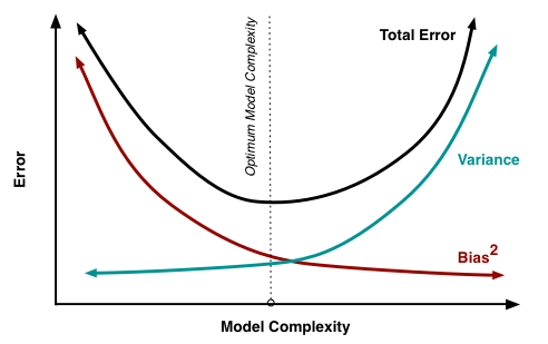
Understanding bias and variance is critical for understanding the behavior of prediction models, but in general what you really care about is overall error, not the specific decomposition. The sweet spot for any model is the level of complexity at which the increase in bias is equivalent to the reduction in variance. Mathematically:
$$ \frac{dBias}{dComplexity} = - \frac{dVariance}{dComplexity} $$
If our model complexity exceeds this sweet spot, we are in effect over-fitting our model; while if our complexity falls short of the sweet spot, we are under-fitting the model. In practice, there is not an analytical way to find this location. Instead we must use an accurate measure of prediction error and explore differing levels of model complexity and then choose the complexity level that minimizes the overall error. A key to this process is the selection of an accurate error measure as often grossly inaccurate measures are used which can be deceptive. The topic of accuracy measures is discussed here but generally resampling based measures such as cross-validation should be preferred over theoretical measures such as Aikake's Information Criteria.
❧
-
The Elements of Statistical Learning. A superb book. ↩
-
The simulated data are purely for demonstration purposes. There is no reason to expect it to accurately reflect what would be observed if this experiment was actually carried out. ↩
-
The k-Nearest Neighbors algorithm described above is a little bit of a paradoxical case. It might seem that the "simplest" and least complex model is the one where k is 1. This reasoning is based on the conceit that having more neighbors be involved in calculating the value of a point results in greater complexity. From a computational standpoint this might be true, but it is more accurate to think of complexity from a model standpoint. The greater the variability of the resulting model, the greater its complexity. From this standpoint, we can see that larger values of k result in lower model complexity. ↩
-
It is important to note that this is only true if you have a robust means of properly utilizing each added covariate or piece of complexity. If you have an algorithm that involves non-convex optimizations (e.g. ones with potential local minima and maxima) adding additional covariates could make it harder to find the best set of model parameters and could actually result in higher bias. However, for algorithms like linear regression with efficient and precise machinery, additional covariates will always reduce bias. ↩