Measuring Error

When building prediction models, the primary goal should be to make a model that most accurately predicts the desired target value for new data. The measure of model error that is used should be one that achieves this goal. In practice, however, many modelers instead report a measure of model error that is based not on the error for new data but instead on the error the very same data that was used to train the model. The use of this incorrect error measure can lead to the selection of an inferior and inaccurate model.

Naturally, any model is highly optimized for the data it was trained on. The expected error the model exhibits on new data will always be higher than that it exhibits on the training data. As example, we could go out and sample 100 people and create a regression model to predict an individual's happiness based on their wealth. We can record the squared error for how well our model does on this training set of a hundred people. If we then sampled a different 100 people from the population and applied our model to this new group of people, the squared error will almost always be higher in this second case.

It is helpful to illustrate this fact with an equation. We can develop a relationship between how well a model predicts on new data (its true prediction error and the thing we really care about) and how well it predicts on the training data (which is what many modelers in fact measure).

$$ True\ Prediction\ Error = Training\ Error + Training\ Optimism $$

Here, Training Optimism is basically a measure of how much worse our model does on new data compared to the training data. The more optimistic we are, the better our training error will be compared to what the true error is and the worse our training error will be as an approximation of the true error.

The Danger of Overfitting

In general, we would like to be able to make the claim that the optimism is constant for a given training set. If this were true, we could make the argument that the model that minimizes training error, will also be the model that will minimize the true prediction error for new data. As a consequence, even though our reported training error might be a bit optimistic, using it to compare models will cause us to still select the best model amongst those we have available. So we could in effect ignore the distinction between the true error and training errors for model selection purposes.

Unfortunately, this does not work. It turns out that the optimism is a function of model complexity: as complexity increases so does optimism. Thus we have a our relationship above for true prediction error becomes something like this:

$$ True\ Prediction\ Error = Training\ Error + f(Model\ Complexity) $$

How is the optimism related to model complexity? As model complexity increases (for instance by adding parameters terms in a linear regression) the model will always do a better job fitting the training data. This is a fundamental property of statistical models ¹. In our happiness prediction model, we could use people's middle initials as predictor variables and the training error would go down. We could use stock prices on January 1st, 1990 for a now bankrupt company, and the error would go down. We could even just roll dice to get a data series and the error would still go down. No matter how unrelated the additional factors are to a model, adding them will cause training error to decrease.

But at the same time, as we increase model complexity we can see a change in the true prediction accuracy (what we really care about). If we build a model for happiness that incorporates clearly unrelated factors such as stock ticker prices a century ago, we can say with certainty that such a model must necessarily be worse than the model without the stock ticker prices. Although the stock prices will decrease our training error (if very slightly), they conversely must also increase our prediction error on new data as they increase the variability of the model's predictions making new predictions worse. Furthermore, even adding clearly relevant variables to a model can in fact increase the true prediction error if the signal to noise ratio of those variables is weak.

Let's see what this looks like in practice. We can implement our wealth and happiness model as a linear regression. We can start with the simplest regression possible where $ Happiness=a+b\ Wealth+\epsilon $ and then we can add polynomial terms to model nonlinear effects. Each polynomial term we add increases model complexity. So we could get an intermediate level of complexity with a quadratic model like $Happiness=a+b\ Wealth+c\ Wealth^2+\epsilon$ or a high-level of complexity with a higher-order polynomial like $Happiness=a+b\ Wealth+c\ Wealth^2+d\ Wealth^3+e\ Wealth^4+f\ Wealth^5+g\ Wealth^6+\epsilon$.

The figure below illustrates the relationship between the training error, the true prediction error, and optimism for a model like this. The scatter plots on top illustrate sample data with regressions lines corresponding to different levels of model complexity.

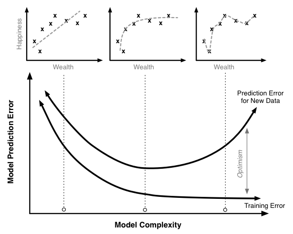
Increasing the model complexity will always decrease the model training error. At very high levels of complexity, we should be able to in effect perfectly predict every single point in the training data set and the training error should be near 0. Similarly, the true prediction error initially falls. The linear model without polynomial terms seems a little too simple for this data set. However, once we pass a certain point, the true prediction error starts to rise. At these high levels of complexity, the additional complexity we are adding helps us fit our training data, but it causes the model to do a worse job of predicting new data.

This is a case of overfitting the training data. In this region the model training algorithm is focusing on precisely matching random chance variability in the training set that is not present in the actual population. We can see this most markedly in the model that fits every point of the training data; clearly this is too tight a fit to the training data.

Preventing overfitting is a key to building robust and accurate prediction models. Overfitting is very easy to miss when only looking at the training error curve. To detect overfitting you need to look at the true prediction error curve. Of course, it is impossible to measure the exact true prediction curve (unless you have the complete data set for your entire population), but there are many different ways that have been developed to attempt to estimate it with great accuracy. The second section of this work will look at a variety of techniques to accurately estimate the model's true prediction error.

An Example of the Cost of Poorly Measuring Error

Let's look at a fairly common modeling workflow and use it to illustrate the pitfalls of using training error in place of the true prediction error ². We'll start by generating 100 simulated data points. Each data point has a target value we are trying to predict along with 50 different parameters. For instance, this target value could be the growth rate of a species of tree and the parameters are precipitation, moisture levels, pressure levels, latitude, longitude, etc. In this case however, we are going to generate every single data point completely randomly. Each number in the data set is completely independent of all the others, and there is no relationship between any of them.

For this data set, we create a linear regression model where we predict the target value using the fifty regression variables. Since we know everything is unrelated we would hope to find an R² of 0. Unfortunately, that is not the case and instead we find an R² of 0.5. That's quite impressive given that our data is pure noise! However, we want to confirm this result so we do an F-test. This test measures the statistical significance of the overall regression to determine if it is better than what would be expected by chance. Using the F-test we find a p-value of 0.53. This indicates our regression is not significant.

If we stopped there, everything would be fine; we would throw out our model which would be the right choice (it is pure noise after all!). However, a common next step would be to throw out only the parameters that were poor predictors, keep the ones that are relatively good predictors and run the regression again. Let's say we kept the parameters that were significant at the 25% level of which there are 21 in this example case. Then we rerun our regression.

In this second regression we would find:

• An R² of 0.36
• A p-value of 5*10^-4
• 6 parameters significant at the 5% level

Again, this data was pure noise; there was absolutely no relationship in it. But from our data we find a highly significant regression, a respectable R² (which can be very high compared to those found in some fields like the social sciences) and 6 significant parameters!

This is quite a troubling result, and this procedure is not an uncommon one but clearly leads to incredibly misleading results. It shows how easily statistical processes can be heavily biased if care to accurately measure error is not taken.

Methods of Measuring Error

Adjusted R²

The R² measure is by far the most widely used and reported measure of error and goodness of fit. R² is calculated quite simply. First the proposed regression model is trained and the differences between the predicted and observed values are calculated and squared. These squared errors are summed and the result is compared to the sum of the squared errors generated using the null model. The null model is a model that simply predicts the average target value regardless of what the input values for that point are. The null model can be thought of as the simplest model possible and serves as a benchmark against which to test other models. Mathematically:

$$ R^2 = 1 - \frac{Sum\ of\ Squared\ Errors\ Model}{Sum\ of\ Squared\ Errors\ Null\ Model} $$

R² has very intuitive properties. When our model does no better than the null model then R² will be 0. When our model makes perfect predictions, R² will be 1. R² is an easy to understand error measure that is in principle generalizable across all regression models.

Commonly, R² is only applied as a measure of training error. This is unfortunate as we saw in the above example how you can get high R² even with data that is pure noise. In fact there is an analytical relationship to determine the expected R² value given a set of n observations and p parameters each of which is pure noise:

$$E\left[R^2\right]=\frac{p}{n}$$

So if you incorporate enough data in your model you can effectively force whatever level of R² you want regardless of what the true relationship is. In our illustrative example above with 50 parameters and 100 observations, we would expect an R² of 50/100 or 0.5.

One attempt to adjust for this phenomenon and penalize additional complexity is Adjusted R². Adjusted R² reduces R² as more parameters are added to the model. There is a simple relationship between adjusted and regular R²:

$$Adjusted\ R^2=1-(1-R^2)\frac{n-1}{n-p-1}$$

Unlike regular R², the error predicted by adjusted R² will start to increase as model complexity becomes very high. Adjusted R² is much better than regular R² and due to this fact, it should always be used in place of regular R². However, adjusted R² does not perfectly match up with the true prediction error. In fact, adjusted R² generally under-penalizes complexity. That is, it fails to decrease the prediction accuracy as much as is required with the addition of added complexity.

Given this, the usage of adjusted R² can still lead to overfitting. Furthermore, adjusted R² is based on certain parametric assumptions that may or may not be true in a specific application. This can further lead to incorrect conclusions based on the usage of adjusted R².

Pros

• Easy to apply
• Built into most existing analysis programs
• Fast to compute
• Easy to interpret ³

Cons

• Less generalizable
• May still overfit the data

Information Theoretic Approaches

There are a variety of approaches which attempt to measure model error as how much information is lost between a candidate model and the true model. Of course the true model (what was actually used to generate the data) is unknown, but given certain assumptions we can still obtain an estimate of the difference between it and and our proposed models. For a given problem the more this difference is, the higher the error and the worse the tested model is.

Information theoretic approaches assume a parametric model. Given a parametric model, we can define the likelihood of a set of data and parameters as the, colloquially, the probability of observing the data given the parameters ⁴. If we adjust the parameters in order to maximize this likelihood we obtain the maximum likelihood estimate of the parameters for a given model and data set. We can then compare different models and differing model complexities using information theoretic approaches to attempt to determine the model that is closest to the true model accounting for the optimism.

The most popular of these the information theoretic techniques is Akaike's Information Criteria (AIC). It can be defined as a function of the likelihood of a specific model and the number of parameters in that model:

$$ AIC = -2 ln(Likelihood) + 2p $$

Like other error criteria, the goal is to minimize the AIC value. The AIC formulation is very elegant. The first part ($-2 ln(Likelihood)$) can be thought of as the training set error rate and the second part ($2p$) can be though of as the penalty to adjust for the optimism.

However, in addition to AIC there are a number of other information theoretic equations that can be used. The two following examples are different information theoretic criteria with alternative derivations. In these cases, the optimism adjustment has different forms and depends on the number of sample size (n).

$$ AICc = -2 ln(Likelihood) + 2p + \frac{2p(p+1)}{n-p-1} $$

$$ BIC = -2 ln(Likelihood) + p\ ln(n) $$

The choice of which information theoretic approach to use is a very complex one and depends on a lot of specific theory, practical considerations and sometimes even philosophical ones. This can make the application of these approaches often a leap of faith that the specific equation used is theoretically suitable to a specific data and modeling problem.

Pros

• Easy to apply
• Built into most advanced analysis programs

Cons

• Metric not comparable between different applications
• Requires a model that can generate likelihoods ⁵
• Various forms a topic of theoretical debate within the academic field

Holdout Set

Both the preceding techniques are based on parametric and theoretical assumptions. If these assumptions are incorrect for a given data set then the methods will likely give erroneous results. Fortunately, there exists a whole separate set of methods to measure error that do not make these assumptions and instead use the data itself to estimate the true prediction error.

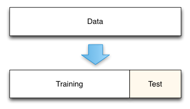
The simplest of these techniques is the holdout set method. Here we initially split our data into two groups. One group will be used to train the model; the second group will be used to measure the resulting model's error. For instance, if we had 1000 observations, we might use 700 to build the model and the remaining 300 samples to measure that model's error.

This technique is really a gold standard for measuring the model's true prediction error. As defined, the model's true prediction error is how well the model will predict for new data. By holding out a test data set from the beginning we can directly measure this.

The cost of the holdout method comes in the amount of data that is removed from the model training process. For instance, in the illustrative example here, we removed 30% of our data. This means that our model is trained on a smaller data set and its error is likely to be higher than if we trained it on the full data set. The standard procedure in this case is to report your error using the holdout set, and then train a final model using all your data. The reported error is likely to be conservative in this case, with the true error of the full model actually being lower. Such conservative predictions are almost always more useful in practice than overly optimistic predictions.

One key aspect of this technique is that the holdout data must truly not be analyzed until you have a final model. A common mistake is to create a holdout set, train a model, test it on the holdout set, and then adjust the model in an iterative process. If you repeatedly use a holdout set to test a model during development, the holdout set becomes contaminated. Its data has been used as part of the model selection process and it no longer gives unbiased estimates of the true model prediction error.

Pros

• No parametric or theoretic assumptions
• Given enough data, highly accurate
• Very simple to implement
• Conceptually simple

Cons

• Potential conservative bias
• Tempting to use the holdout set prior to model completion resulting in contamination
• Must choose the size of the holdout set (70%-30% is a common split)

Cross-Validation and Resampling

In some cases the cost of setting aside a significant portion of the data set like the holdout method requires is too high. As a solution, in these cases a resampling based technique such as cross-validation may be used instead.

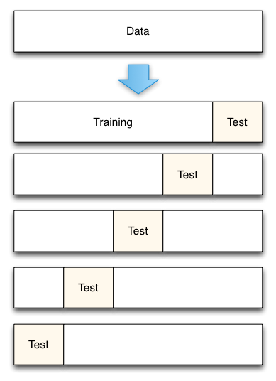
Cross-validation works by splitting the data up into a set of n folds. So, for example, in the case of 5-fold cross-validation with 100 data points, you would create 5 folds each containing 20 data points. Then the model building and error estimation process is repeated 5 times. Each time four of the groups are combined (resulting in 80 data points) and used to train your model. Then the 5th group of 20 points that was not used to construct the model is used to estimate the true prediction error. In the case of 5-fold cross-validation you would end up with 5 error estimates that could then be averaged to obtain a more robust estimate of the true prediction error.

As can be seen, cross-validation is very similar to the holdout method. Where it differs, is that each data point is used both to train models and to test a model, but never at the same time. Where data is limited, cross-validation is preferred to the holdout set as less data must be set aside in each fold than is needed in the pure holdout method. Cross-validation can also give estimates of the variability of the true error estimation which is a useful feature. However, if understanding this variability is a primary goal, other resampling methods such as Bootstrapping are generally superior.

On important question of cross-validation is what number of folds to use. Basically, the smaller the number of folds, the more biased the error estimates (they will be biased to be conservative indicating higher error than there is in reality) but the less variable they will be. On the extreme end you can have one fold for each data point which is known as Leave-One-Out-Cross-Validation. In this case, your error estimate is essentially unbiased but it could potentially have high variance. Understanding the Bias-Variance Tradeoff is important when making these decisions. Another factor to consider is computational time which increases with the number of folds. For each fold you will have to train a new model, so if this process is slow, it might be prudent to use a small number of folds. Ultimately, it appears that, in practice, 5-fold or 10-fold cross-validation are generally effective fold sizes.

Pros

• No parametric or theoretic assumptions
• Given enough data, highly accurate
• Conceptually simple

Cons

• Computationally intensive
• Must choose the fold size
• Potential conservative bias

Making a Choice

In summary, here are some techniques you can use to more accurately measure model prediction error:

• Adjusted R²
• Information Theoretic Techniques
• Holdout Sample
• Cross-Validation and Resampling Methods

A fundamental choice a modeler must make is whether they want to rely on theoretic and parametric assumptions to adjust for the optimism like the first two methods require. Alternatively, does the modeler instead want to use the data itself in order to estimate the optimism.

Generally, the assumption based methods are much faster to apply, but this convenience comes at a high cost. First, the assumptions that underly these methods are generally wrong. How wrong they are and how much this skews results varies on a case by case basis. The error might be negligible in many cases, but fundamentally results derived from these techniques require a great deal of trust on the part of evaluators that this error is small.

Ultimately, in my own work I prefer cross-validation based approaches. Cross-validation provides good error estimates with minimal assumptions. The primary cost of cross-validation is computational intensity but with the rapid increase in computing power, this issue is becoming increasingly marginal. At its root, the cost with parametric assumptions is that even though they are acceptable in most cases, there is no clear way to show their suitability for a specific case. Thus their use provides lines of attack to critique a model and throw doubt on its results. Although cross-validation might take a little longer to apply initially, it provides more confidence and security in the resulting conclusions.